当模拟真实世界数据用于回归分析时,我们观察到,很少情况下,模型的方程是给出线性图的线性方程。大多数时候,真实世界数据模型的方程涉及更高程度的数学函数,如3的指数或sin函数。在这种情况下,模型的图给出了曲线而不是线。线性和非线性回归的目的是调整模型参数的值,以找到最接近您的数据的线或曲线。在找到这些值时,我们将能够以良好的精确度估计响应变量。
在最小二乘回归中,我们建立了一个回归模型,其中来自回归曲线的不同点的垂直距离的平方和被最小化。我们通常从定义的模型开始,并假设系数的一些值。然后我们应用R语言的nls()函数获得更准确的值以及置信区间。
语法
在R语言中创建非线性最小二乘测试的基本语法是 -
nls(formula, data, start)
以下是所使用的参数的描述 -
formula是包括变量和参数的非线性模型公式。
data是用于计算公式中变量的数据框。
start是起始估计的命名列表或命名数字向量。
例
我们将考虑一个假设其系数的初始值的非线性模型。 接下来,我们将看到这些假设值的置信区间是什么,以便我们可以判断这些值在模型中有多好。
所以让我们考虑下面的方程为这个目的 -
a = b1*x^2+b2
让我们假设初始系数为1和3,并将这些值拟合到nls()函数中。
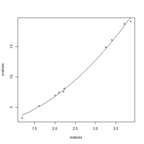
xvalues <- c(1.6,2.1,2,2.23,3.71,3.25,3.4,3.86,1.19,2.21)
yvalues <- c(5.19,7.43,6.94,8.11,18.75,14.88,16.06,19.12,3.21,7.58)

# Give the chart file a name.
png(file = "nls.png")


# Plot these values.
plot(xvalues,yvalues)


# Take the assumed values and fit into the model.
model <- nls(yvalues ~ b1*xvalues^2+b2,start = list(b1 = 1,b2 = 3))

# Plot the chart with new data by fitting it to a prediction from 100 data points.
new.data <- data.frame(xvalues = seq(min(xvalues),max(xvalues),len = 100))
lines(new.data$xvalues,predict(model,newdata = new.data))

# Save the file.
dev.off()

# Get the sum of the squared residuals.
print(sum(resid(model)^2))

# Get the confidence intervals on the chosen values of the coefficients.
print(confint(model))
当我们执行上面的代码,它产生以下结果 -
[1] 1.081935
Waiting for profiling to be done...
       2.5%    97.5%
b1 1.137708 1.253135
b2 1.497364 2.496484
我们可以得出结论,b1的值更接近1,而b2的值更接近2而不是3。