中国教程网zhangditony翻译,转载请保留此信息 .
1. Sort the List by Customer Name by selecting a cell in column C and clicking the Sort icon.(按客户排序)
2. Select cell A1 in the Current Region and press Ctrl+Shift+*(按ctrl+shift+*选择排序后区域)
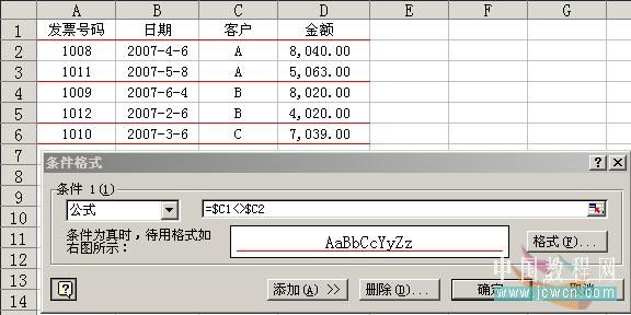
3. From the Format menu, select Conditional Formatting.(选格式-条件格式)
4. In Condition 1, select Formula Is.
5. In the Formula box, enter the formula =$C1$C2. Be sure to enter the formula with absolute reference for the column and relative reference for the row.(输入公式=$C1$C2,注意绝对引用及相对引用)
6. In the Conditional Formatting dialog box, click the Format button, select the Border tab, in Border section click Underline and then choose a color.(在条件格式中的格式对话框,选择边框中的下边框及颜色)
7. Click OK twice.(按确定)
